It is time to address a small problem… The image processing that I apply after rendering the 3D models for the characters is too slow. I mean, 2.42 seconds per image does not look like too much but if you take into account that we will have to process around 30.000 images it starts adding up.
The different parts of the image processing are:
- Reading the image: this part is done by the skimage package so we will not worry about the speed of this part.
- Down-scaling image: to downscale the image we also use a function of the skimage package that is really fast, so we won’t worry about this part.
- Reducing the amount of colours: this is a custom function that uses numpy arrays operations to reduce the amount of colours as much as possible without being noticeable for the human eye.
- Getting the colours of the palette: this function reads an image and creates a list with its colours. Since this function is just used once in every batch of images it is not a problem and it is already quite fast.
- Remapping the colours of the image: this is the most important function and the one that takes most of the time. What it does is changing the colours of one image for the closest one in a palette.
Benchmarks
To do the benchmarks I am using my own laptop, that usually is running more process in the background. The benchmark consist in processing 25 images with an input resolution of 640x900 to an output resolution of 64x90 with a palette of 47 colours. To reduce the image colours we are using a maximum distance of 18, which in the test has shown to work good enough.
Yes, it is not the best benchmark in the world, in fact is bad, but it should be good enough. These are the results:
| Functions | Time |
|---|---|
| load | 0.475 |
| downscale | 0.462 |
| reduce colours | 8.575 |
| get colours | 0.000181 |
| remap colours | 49.290 |
As you can see the two functions that deserve our attention is the colour reduction and the colour remapping ones. I don’t know how I managed to create such a slow code. Each image takes 2.42s to be processed.
The new approach will be based on the idea of instead of creating a function that will return us the colour reduced image we will create a function that returns the reduced colour palette. Then we could use the colour remapping function to apply this reduced palette to the image and after that the new palette.
Colour reduction
This is the code that I am using right now:
def reduce_colors(img, threshold):
    # First we create a empty list of colours
    colors = list()
	# Then we iterate through all the pixels
    for y, row in enumerate(img):
        for x, pixel in enumerate(row):
           	# We iterate over all the colours to get the
            # index of the closest colour
            dist = float("inf")
            index = 0
            for pos, color in enumerate(colors):
                new_dist = np.linalg.norm(color-pixel)
                if new_dist < dist:
                    dist = new_dist
                    index = pos
            # If the distance is bigger than the threshold we add
            # the colour to the list of colours. If this is not the
            # case we change the colour to the closest one.
            if dist > threshold:
                colors.append(pixel)
            else:
                img[y][x] = colors[index]

    return img
Yes, this code could have been done by a monkey, but I needed to make sure that this approach worked before worrying about how fast it was. I also know it is not the best way to do it because it just has into account the first occurrence of the colour and not the average of all the colours that are under the threshold. This is an example of the images I am working with:

The biggest problem is that we are following an iterative approach by using 3 for loops when numpy is optimised for matrix operations. Seriously, this code is plain garbage, I am ashamed of myself, but we are still in time to amend our mistakes.
Getting the reduced palette
At this point we don’t care about the geometry of the image so we could imagine that it is just a list of colours… A set of points in a 4D space (we are working with an RGBA colour model)… Okay, what if we use a clustering technique and the calculate the centroid (average) of all the members of the cluster? First of all, this approach should be way faster and secondly it solves the problem of taking just the first element.
First problem: which clustering algorithm to use. In order to find the answer lets refer to this document from scikit learn: 2.3. Clustering.
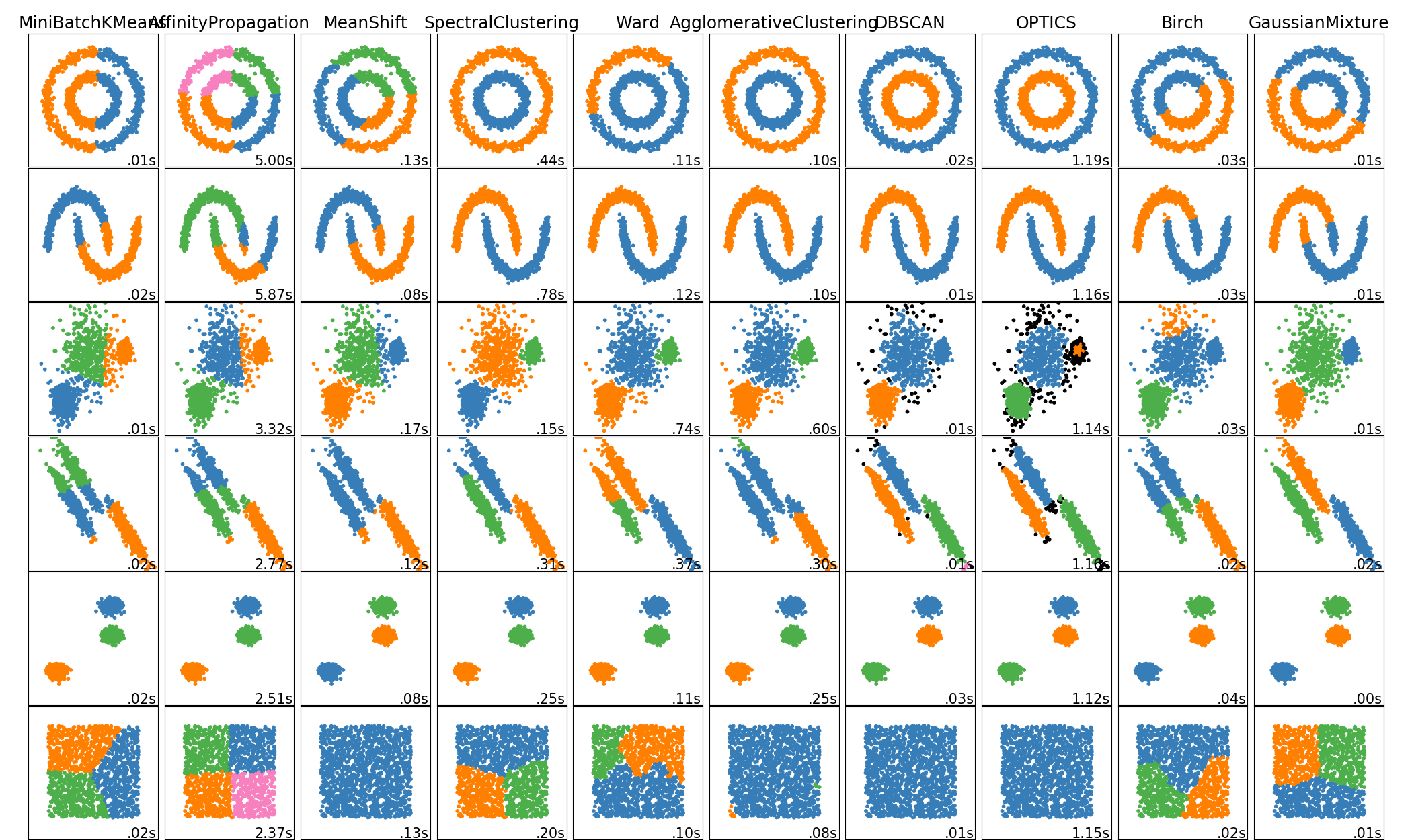
Our data will have a shape similar to the fifth row and the speed shouldn’t be a problem since this package is really fast. The most important thing to have into account is that we don’t know the number of clusters that we will need so our loved K-Means is out of the game. After trying multiple options with different images the one that has given the best results is Mean Shift.
Before applying the clustering algorithm we should think if it is possible to process our data to improve the speed. As I said before we are using a RGBA model and in our image the alpha value is either 0 or 255. This is because when we downscale our image we disable the anti-aliasing to get this pixel-art effect. Since all the values with 0 alpha belong to the background and we don’t care about them we can delete all the members of our dataset that have 0 alpha and after that we can reduce the dimensionality to 3 by deleting the alpha value of all our members.
Let’s see how we can do this:
import numpy as np

# Reshape the data
data = img.reshape(img.shape[0]*img.shape[1],img.shape[2])
# Delete transparent pixels and reduce dimensions to 3
data = data[data[:,3] != 0]
data = data[:,0:3]
Using a real image like the ones we are going to process for the real game we have reduced the amount of values from 23040 (64 * 90 * 4) to 2997 (999 * 3). Now it is time to apply the Mean Shift algorithm. We will use scikit-learn package for that:
from sklearn.cluster import MeanShift, estimate_bandwidth

# calculate clusters and centroids
bandwidth = estimate_bandwidth(data, quantile=0.14, n_samples=len(data))
ms = MeanShift(bandwidth=bandwidth, bin_seeding=True).fit(data)
palette = ms.cluster_centers_.astype(np.uint8)
And by accessing ms.cluster_centers_ we can get the centroids of the clusters. The quantile value has been decided based on experimentation with different images of the set we are going to work with.
Colour remapping
Now we have a colour palette and an image, so we have to think how to apply this colour palette. The RGB colour model is oriented to the user and uniform, this means that it is based in how humans perceive the colours and that the difference between how humans percieve two colours can be calculated using the euclidean distance inside a 3D space. This means that the smaller the euclidean distance, the more similar are the colours, so we will have to find the euclidean distance between each pixel with all the colours and choose the one with the smallest.
This is how I decided to implement the distance calculation:
from scipy.spatial.distance import cdist

# Calculate distances
distances = cdist(data, palette)
# Get the index of the color with minimun distance
index_nearest_colour = np.argmin(distances,axis=1)
# Create a list with the colours with the minimum distances
out_rgb = palette[indexes]
But this array is not usable yet. First we have to add the alpha value again and add all the transparent pixels we removed at the beginning:
# Add alpha value
out_rgba = np.ones((out_rgb.shape[0],out_rgb.shape[1]+1))*255
out_rgba[:,:-1] = out_rgb

# Put the colours in the places where they belong
index_not_transparent = np.where(img[:,:,3] != 0)
img_out = np.zeros_like(img)
img_out[index_not_transparent[0][:],index_not_transparent[1][:]] = out_rgba[:]
And that’s all, we have an image with a reduced amount of different colours.
A step further
Now we have a set of really cool functions that allow us to extract palettes from images and apply them to other images. The only thing that we have to do now is to iterate over all the images and one by one extract the reduced colour palette and remap the image with this palette… No. Wrong. We have to take into account the properties of our data. Since we are working with sets of images that represent the same character in different positions and from different angles the colour palette should be the same. We can combine all our data that comes from the same character, extract the colour palette once and then apply it to all our images. This should be faster and give us better results. Lets see how do we do it:
# Origin and destination are strings with paths to the folders
files = [f for f in listdir(origin) if isfile(join(origin, f))]
image_collection = np.empty(shape=(len(files),90,64,4))

# Store all the images in one array
for pos,image_path in enumerate(files):
    img = skimage.io.imread(origin + '/' + image_path)
    img = downscale(img)
    image_collection[pos] = img

# Extract the important data and calculate the reduced colour palette
data = image2data(image_collection)
data_shuffle = np.random.permutation(data)
reduced_palette = reduce_colours(data_shuffle[:2000])

# Remap the data and convert it to a usable image
data = remap_colours(data, reduced_palette)
data = remap_colours(data, new_palette)
img = data2image(data,image_collection.reshape(90,-1,4)).reshape(-1,90,64,4)

# Save the images
for pos,image in enumerate(img):
	skimage.io.imsave(destination + '/' + files[pos], image)
Benchmarks
Okay, now let’s have a look to the time of executing all the process with different amounts of images. In this graph we can see the times of the code above compared to a iterative version of the same where each image is processed completely individually:
-1591031078701.svg)
As we can see, at least in the first half, both approaches are linear, but the iterative process has a bigger inclination. The difference in time is huge. If we compare the times for 3000 images (that is the size of the sets of images that we are going to work with ) the iterative approach takes 138.34 s while the combined approach takes 22.5. This is 6.15 times faster. By the way, the original code would have taken 7260 s approx, this means that our code now it is 322.66 times faster.
But what happens on the second half of the graph? This problem drove me crazy. For some reason during the tests I was seeing that the combined approach had a quadratic cost. At some point I thought that it was because since in this approach we load all the images at the beginning maybe the reading speed of the discs was causing it to slow down because it was not fast enough (remember that in the iterative approach the images are loaded one after the other, so it should not be affected by this problem). I made some more tests and found out that the problem was in the load of the images but not because of my disk, but because of my code. A previous version of my code looked like this:
image_collection = np.empty(shape=(0,90,64,4))

for image_path in files:
    img = skimage.io.imread(origin + '/' + image_path)
    img = downscale(img)
    img = img.reshape(1,90,64,4)
    image_collection = np.append(image_collection,img,axis=0)
It turns out that appending is not as good option as it looked at the beginning. It is better to create the array with the final size and then just replace the data.
I thought the problem was solved, but when I made tests with larges amount of data (more than 10.000 images) it was still showing a quadratic behaviour. I tried to write to a friend about my problem and the computer was so slow that I was not able to do it. But the CPU usage meter at the top of my screen was showing the expected 25% of usage (just one thread). I ran top and I saw the problem, it was the memory. My main and swap memory where full. Since 10.000 images is way more than the amount of images I will work with I am not solving this problem, but the solution should be as simple as dividing the set of images on multiple subsets so the memory can be freed after each subset.
Conclusion
Is this the best way to do it? No. There are still things that can be made to improve the performance, like parallelize the load and saving of the images or dividing the set of images on subsets so we do not run out of resources in the system. The benchmark also should be better. It is horrible. A better way to do it would be to create a set of images with different colours, introduce some noise and the compare the difference between the images.
Despite this, I am really happy with the results and I don’t think it is worth to invest more time, even I have to admit that I had lot of fun working in this problem.
Appendix A: tidy code
from scipy.spatial.distance import cdist
import skimage.io
import skimage.transform
import time
import numpy as np
from tqdm import tqdm
import matplotlib.pyplot as plt
from sklearn.cluster import MeanShift, estimate_bandwidth


def downscale(img):
    img = skimage.transform.resize(img,
                            (90, 64),
                            mode='edge',
                            anti_aliasing=False,
                            anti_aliasing_sigma=None,
                            preserve_range=True,
                            order=0)

    return img


def image2data(img):
    data = img.reshape(img.shape[0]*img.shape[1],img.shape[2])
    data = data[data[:,3] != 0]
    data = data[:,0:3]

    return data


def data2image(data, img):
    rgba = np.ones((data.shape[0],data.shape[1]+1))*255
    rgba[:,:-1] = data
    index_not_transparent = np.where(img[:,:,3] != 0)
    img_out = np.zeros_like(img)
    img_out[index_not_transparent[0][:],index_not_transparent[1][:]] = rgba[:]

    return  img_out


def reduce_colours(data):
    bandwidth = estimate_bandwidth(data, quantile=0.14, n_samples=len(data))
    ms = MeanShift(bandwidth=bandwidth, bin_seeding=True).fit(data)
    palette = ms.cluster_centers_.astype(np.uint8)

    return palette


def remap_colours(data,palette):
    distances = cdist(data, palette)
    indexes_nearest_colour = np.argmin(distances,axis=1)
    data = palette[indexes_nearest_colour]

    return data


def get_colors(img):
    img = img.reshape(img.shape[0]*img.shape[1],img.shape[2])
    ret = np.unique(img,axis=0)[:,:3]

    return ret


def count_colors(img):
    ret = get_colors(img).shape[0]

    return ret